Visualising Instruments

This example demonstrates how to use the show() method on various instrument objects like Camera and Radar to create visualisations. It also shows how to annotate plots with geographical positions.

from matplotlib import pyplot as plt
from arguslib.camera.camera import Camera
import datetime

from arguslib.instruments.instruments import Position
from arguslib.radar.radar import Radar

dt = datetime.datetime(2025, 3, 25, 9)

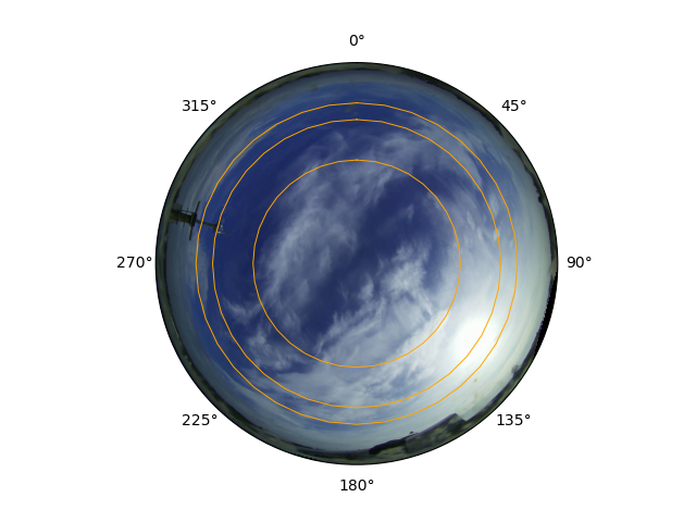
Plotting camera images

Plotting images on a polar plot, with the axes aligned with the ordinal directions.

cam = Camera.from_config("COBALT", "3-7")
cam.show(dt)

<PolarAxes: >

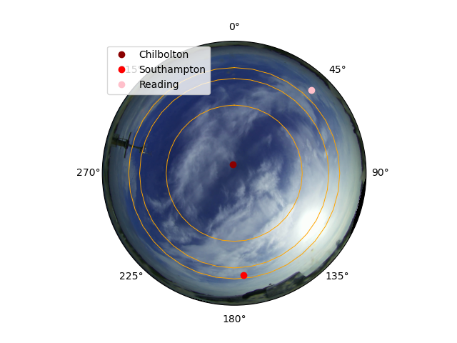
Annotating positions

We can annotate a position on the image. Here, we add a red dot at 10km altitude above Southampton, a pink dot 10km above Reading, and a dark red dot 10km above Chilbolton.

ax = cam.show(dt)
cam.annotate_positions(
    [Position(-1.4419, 51.1553, 10.0)],
    dt,
    ax,
    marker="o",
    lw=0,
    color="darkred",
    label="Chilbolton",
)
cam.annotate_positions(
    [Position(-1.4049, 50.9105, 10.0)],
    dt,
    ax,
    marker="o",
    lw=0,
    color="red",
    label="Southampton",
)
cam.annotate_positions(
    [Position(-0.9783, 51.4550, 10.0)],
    dt,
    ax,
    marker="o",
    lw=0,
    color="pink",
    label="Reading",
)

ax.legend(loc="upper left")

<matplotlib.legend.Legend object at 0x7fe9194157f0>

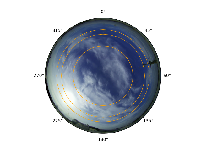
Controlling image orientation

We can also plot the image “unflipped”, either by setting up the axes to be flipped:

cam.show(dt, theta_behaviour="unflipped_ordinal_aligned")

<PolarAxes: >

Or by setting the lr_flip argument to False.

cam.show(
    dt,
    lr_flip=False,
)

<PolarAxes: >

We can set the theta behaviour to be “pixels”, where the theta grid shows the major axes of the pixel grid.

cam.show(dt, theta_behaviour="pixels")

<PolarAxes: >

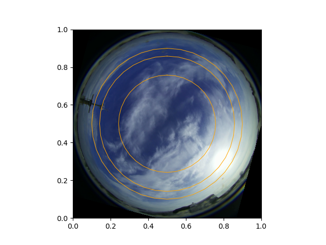
This lines up with the native image grid, which is seen when we plot on non-polar axes.

fig, ax = plt.subplots()
cam.show(dt, ax=ax)

<Axes: >

To still get the rotation, but in place of an existing non-polar set of axes, we can use the replace_ax argument.

fig, ax = plt.subplots()
cam.show(dt, replace_ax=ax)

• 
• 

<PolarAxes: >

The infrastructure can be rigged to plot in a way that doesn’t make sense. Here, we set up a “bearing” axes, but then don’t flip the axes, so the angles don’t line up with the ordinal directions.

cam.show(
    dt,
    theta_behaviour="bearing",
    lr_flip=False,
)

<PolarAxes: >

Plotting radar data

Radar objects can also be plotted using the analogous show function. The axes don’t have so much rotating and flipping to do. Following pyart default behaviour, the positive x direction is towards 0 degrees azimuth (i.e. south to north).

radar = Radar.from_config("COBALT")
radar.show(datetime.datetime(2025, 5, 1, 7, 25, 6), var="DBZ")

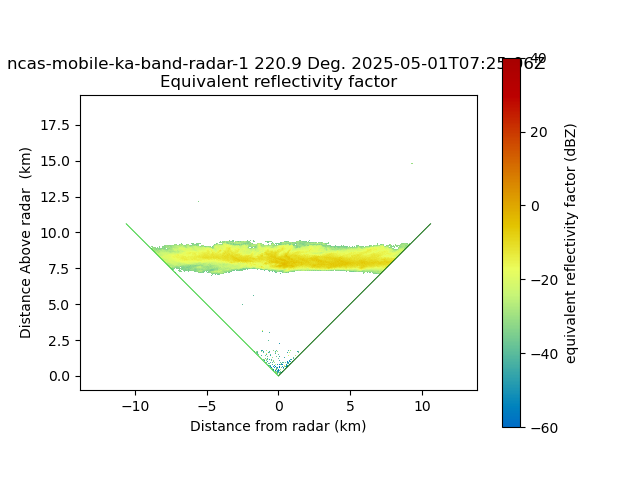
<Axes: title={'center': 'ncas-mobile-ka-band-radar-1 220.9 Deg. 2025-05-01T07:25:06Z \nEquivalent reflectivity factor'}, xlabel='Distance from radar (km)', ylabel='Distance Above radar  (km)'>